
What is PDF? Part 3 – Vector graphis
Categories: Development
Vector graphics
In the third part I cover vector graphics. You can also include PNG and JPEG images in the PDF, which will be covered in a later part of the PDF introduction.
Part 1 – PDF syntax and file structure
Part 2 – Fonts
Part 3 - Vector graphics
Part 4 - Interactive features
Part 5 - Metadata
Please note that all of these examples are created manually. If you wish to experiment with the examples, you can do so yourself. For more information, visit https://github.com/speedata/fixxref which provides a small program that supports manual PDF editing.
What are vector graphics?
Vector graphics are expressed as lines and curves, allowing for sharp and accurate rendering at any size. This means that the rendering will always be sharp and accurate, unless you have a low-resolution output device. Vector graphics typically take up little space in the PDF file. Bitmap graphics, on the other hand, take up a lot of space in the PDF file or may look blurry. There are only a few drawing commands:
| Operator | Meaning |
|---|---|
| m | moveto, move to a certain point in a coordinate system |
| l (lowercase L) | lineto, draw a line from the current position to another position |
| c, v, y | curveto, draw a cubic Bézier curve |
| re | rectangle, draw a rectangle from a given position with a width and a height |
| h | Close the subpath |
All of these commands don’t render anything. For rendering, there are the path painting operators:
| Operator | Meaning |
|---|---|
| S | Stroke the path |
| s | Stroke and close the path |
| f, f* | Fill the path |
| B, B* | Fill and then stroke the path |
| b, b* | Close, fill, and then stroke the path |
| n | End the path without stroking |
The * variants use a different method to find the area to be filled. See this example for the difference (source):
4 0 obj
<<
    /Length 94
>>
stream
1 w
75 150 m 120 8 l 0 96 l 150 96 l 30 8 l
f*

275 150 m 320 8 l 200 96 l 350 96 l 230 8 l
f
endstream
endobj

Colors
I will not go into detail about color spaces in this section. Instead, I will focus on the importance of CMYK (cyan, magenta, yellow, black) and RGB (red, green, blue) colors.
CMYK is crucial in the printing world, while RGB colors are sufficient for on-screen use.
| Operator | Meaning |
|---|---|
| K,k | Set CMYK color for stroking (K) and nonstroking (k) operations. |
| RG, rg | Set RGB color for stroking (RG) and nonstroking (rg) operations. |
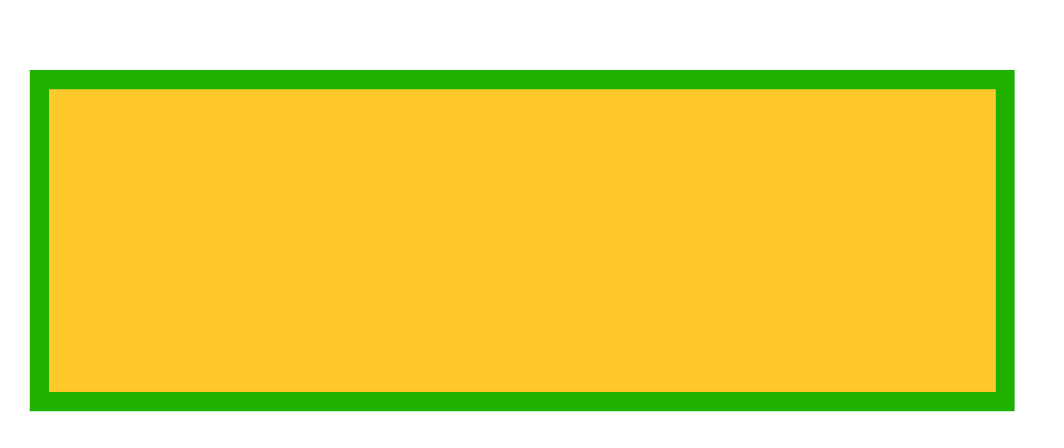
To see the difference between stroking and nonstroking operations consider the following example (source):
4 0 obj
<<
    /Length 195
>>
stream
3 w                  % line width
1 0.782 0.171 rg     % for non stroking
                     %  = filling
0.113 0.694 0.002 RG % stroking
10 10 150 50 re
B                    % Fill and stroke
endstream
endobj
The graphics operators offer numerous possibilities for creating graphics.
Graphics state
Sometimes I need to change some parameters like color and line width and then go back to the previous settings. Luckily there is a push / pop or save / restore mechanism for these settings. To save the graphics state, insert the q operator, to restore, insert Q (source).
4 0 obj
<<
    /Length 299
>>
stream
q                   % save graphics state
3 w
0.113 0.694 0.002 RG
10 10 m 100 10 l s  % green line
Q                   % restore graphics state
10 20 m 100 20 l s  % thin black line: color and line width
                    % settings are back to the (default)
                    % previous state
endstream
endobj

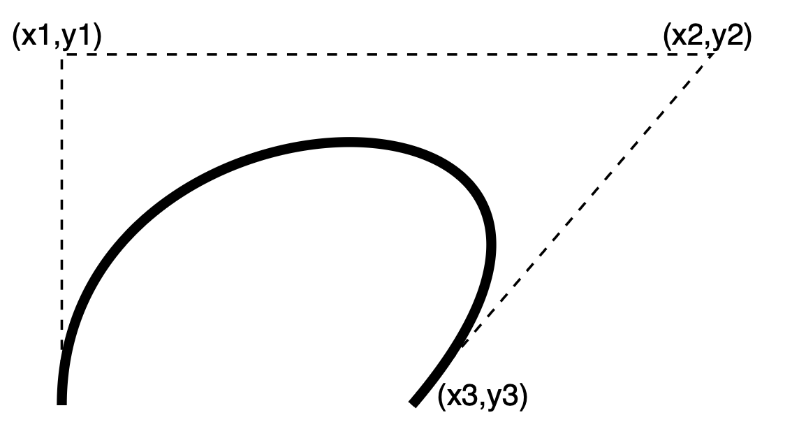
Circles and curves
There are pretty much only two different ways to draw something on the page, a straight line or a (cubic) Bézier curve. See the Wikipedia entry for some math behind the curve. In short: from a starting point (the current position) the curve goes to (x3,y3) and the two points (x1,y1) and (x2,y2) control the shape of the curve (source).
4 0 obj
<<
    /Length 214
>>
stream
2 w
10 10 m
10 80 140 80 80 10 c
S
0.5 w
[ 2 ] 1 d
10 10 m
10 80 l
140 80 l
80 10 l
S
BT
  /F1 6 Tf
  1 0 0 1 0 82 Tm
  (\(x1,y1\)) Tj

  1 0 0 1 130 82 Tm
  (\(x2,y2\)) Tj

  1 0 0 1 85 10 Tm
  (\(x3,y3\)) Tj
ET
endstream
endobj
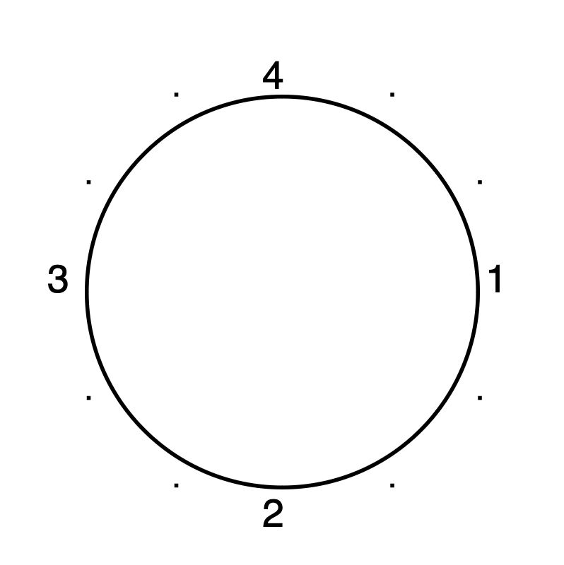
To create a circle in a PDF, you can approximate it by concatenating arcs. The following example demonstrates how four segments can form a circle. The coordinates can be calculated with some non trivial math (I find this non trivial…) (source)
4 0 obj
<<
    /Length 601
>>
stream
150 100 m                          %    point 1
150    72.4 127.6  50   100  50 c  % to point 2
 72.4  50    50    72.4  50 100 c  % to point 3
 50   127.6  72.4 150   100 150 c  % to point 4
127.6 150   150   127.6 150 100 c  % to point 1
S
BT
/F1 10 Tf
  1 0 0 1 152 100 Tm (1) Tj
  1 0 0 1 95 40 Tm (2) Tj
  1 0 0 1 40 100 Tm (3) Tj
  1 0 0 1 95 152 Tm (4) Tj
ET
% control points
% first arc (1-2)
150 72.4 1 1 re f
127.6 50 1 1 re f
% second arc (2-3)
72.4 50 1 1 re f
50 72.4 1 1 re f
% third arc (3-4)
50 127.6 1 1 re f
72.4 150 1 1 re f
% second arc (4-1)
127.6 150 1 1 re f
150 127.6 1 1 re f
endstream
endobj
Clipping
Vector graphics are not only used for drawing lines and curves on the canvas, they can be used to hide contents (clipping) (source).
4 0 obj
<<
    /Length 162
>>
stream
% the star
75 150 m 120 8 l 0 96 l 150 96 l 30 8 l h
W % use this path for clipping
S % use 'n' instead of 'S' to hide the star
% a small square
30 30 90 90 re f
endstream
endobj

Clipping is also part of the graphics state. So you can limit the effect of clipping with q and Q.
For example when I insert a q before drawing the star and a Q right after the S, the following rectangle is not clipped by the path.
Transformation (scaling, rotation, …)
With some math, you can transform objects (or more precise: coordinate systems). Transformations are expressed as six numbers $a$, $b$, $c$, $d$, $e$, $f$ that relate to the equations
$$ 𝑥’ = a \cdot 𝑥 + c \cdot 𝑦 + e \\ 𝑦’ = b \cdot 𝑥 + d \cdot 𝑦 + f $$
The default values are $1$, $0$, $0$, $1$, $0$, $0$ for the “identity transformation”, so the formula evaluates to
$$ 𝑥’ = 1 \cdot 𝑥 + 0 \cdot 𝑦 + 0 \\ 𝑦’ = 0 \cdot 𝑥 + 1 \cdot 𝑦 + 0 $$
You can see that the last two numbers $e$ and $f$ are for shifting in x and y coordinates. Let me show you how to apply the transformation in practice (source):
4 0 obj
<<
    /Length 45
>>
stream
0.8 0.8 0.17 0.8 -10 0 cm
10 10 100 100 re
F
endstream
endobj

First I set the transformation matrix with the command cm. Every object following the transformation command is drawn in the new coordinate system.
There are some common transformations:
- Translations are specified with the values $1$, $0$, $0$, $1$, $t_x$ and $t_y$, where $t_x$ and $t_y$ are the horizontal and vertical offsets in DTP points.
- Scaling can be achieved with the values $s_x$, $0$, $0$, $s_y$, $0$ and $0$. This scales the coordinate system by the given amount (1 = no scaling)
- Rotation can be get by $\cos θ$, $\sin θ$, $−\sin θ$, $\cos θ$, $0$ and $0$ (counter clockwise).
- Skew is specified by $1$, $\tan α$, $\tan β$, $1$, $0$ and $0$, which skews the x axis by an angle $α$ and the y axis by an angle $β$.
I know that this is very a bit short, you can find all the details about coordinate systems in the PDF spec in section 4.2.2 (PDF 1.7) or 8.3.3 (PDF 2.0).